How to Use Computer Vision in Cancer Research With MLOps
We introduced Picsellia's new features by presenting a cancer cell research real use-case. Learn how we applied computer vision to medical research.
Picsellia Team
·16 min read
Put your MLOps into practice
Stop stitching tools together. Get an end-to-end CV platform with built-in automation.
We casted a webinar to introduce the new version of our platform, now centered on MLOps, and more precisely, on CVOps–MLOps applied computer vision. At Picsellia, we offer an end-to-end computer vision (CV) platform that lets you manage AI data, run experiments, deploy models into production and monitor them with automated pipelines.
To introduce you to Picsellia’s new features, we’ve prepared a use-case in collaboration with the Toulouse Cancer Research Center. If you’d like to watch a replay of our webinar, it’s available on youtube, right here!
Summary
- About the use-case
- Annotating your dataset
- Training your model
- Launching the experiment
- Exporting the model
- Deploying the model
- Making predictions/inferences
- Training a model on a custom dataset of fibroblast nucleus
- Continuous training and alert system
- Comparing shadow models
About the use-case
The use-case was possible thanks to the Toulouse Cancer Research Center, whose collaborators shared with us some of their obstacles for testing and researching.
The center is studying the propagation of cancer cells under microscopes, and researching how some other cells that are natively in our body, called fibroblasts, are helping cancer propagate.
Nowadays, what scientists measure regarding propagation is global fluorescence. By activating some enzymes on the cells, they can monitor the global fluorescence of an image. But, this fluorescence must be reported to the number of cells in the photo to have significant results.
Just counting the cells of an image, can take from 2–3 hours, up to 10–12 hours a week, hampering their research process.
At Picsellia, we thought that AI and computer vision could help them in detecting those cells’ nucleus and automating the cell counting process, bringing the 10-hour counting process to something like 2–3 minutes for a thousand of images.
Methodology
In short, we’ll try to train a new model that will serve as a base-model on our dataset, and we will fine tune it and use it to pre-annotate our images and see how it performs. Our dataset was suited for segmentation but we will use it for object detection just to make the use case simpler, and because object detection is suited for cell counting.
Annotating your dataset
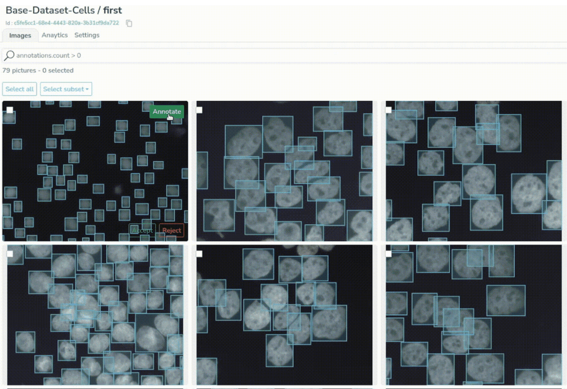
We’ll start in the data lake. This is where all the assets stored can be viewed and searched, for example by tag or other attributes.
Here we have many more images than needed for our use case so we’re going to filter only the images from the Nature dataset, by the tag “nature”.
 How to use computer vision in cancer research 66ed39473bd1d937d97be4bb 623c46bc0f775651c366e8b3 ex1
We see that we only list 79 images, which is the size of the original dataset. We can also switch to a list view and see the filename and attributes of images.
 How to use computer vision in cancer research 6242b9cdee28fe449701f700 0 gxash6zam3vqz1df
Now we need to select them all and create a Picsellia dataset that we’ll call “empty_images”.
 How to use computer vision in cancer research 66ed39473bd1d937d97be4be 6242b9ee0bf24e89a32ce8df exhibit 25202
As it should be created now, we can head to the dataset. Let’s select the dataset we want and the “empty_images” version we just created.
 How to use computer vision in cancer research 66ed39473bd1d937d97be4c1 6242ba0db21bef701f8a0cac exhibit 3
In a dataset, you can import annotations. As the nature dataset was already labeled, we imported the annotations into a new version of our dataset.
 How to use computer vision in cancer research 6242ba2073d2736e28eff82b 0 943k9zfwxmtxj4cp
We go back to our datasets, and choose the one that is already annotated.
 How to use computer vision in cancer research 6242ba312b2dda8c6d29aee6 0 ouovd8 lplh6edu
Once there, we can visualize all the annotations that were made. The consistency looks pretty good and all the cells are labeled.
 How to use computer vision in cancer research 6242ba40618a91fce0dfa6b4 0 n3hxszbpnjo8ui8y
If we select one image and go to our annotation tool, if needed, we can edit the annotations one by one, or create a new annotation with our collaborative annotation interface.
 How to use computer vision in cancer research 66ed39473bd1d937d97be4c8 6242ba67ee28fe792e01f8d0 exhibit 4
As shown next, in the data lake you can filter your images by attribute, including objects in the annotations. For example, we can choose to visualize all the images that contain more than 20 cells annotated, and see that it narrows down the number of images to 56.
 How to use computer vision in cancer research 66ed39473bd1d937d97be559 6242bace771207efd643d5cf exhibit 5
Training Your Model
Now that we are happy with our fully annotated dataset, we can move on to model training.
Let’s create a new project. We’ll call it base-nature-cells, invite our team, and validate it.
 How to use computer vision in cancer research 66ed39463bd1d937d97be3b8 6242bb53734c0a71e5ae31f5 exhibibt 6 1
Next, we’ll attach the dataset we just created (with the annotations) to our project, and that will be the source of the experiment we’ll create right now.
 How to use computer vision in cancer research 66ed39473bd1d937d97be4cb 6242bb956cd7610415121296 exhibit 7
Let’s call it v0 and choose in our model HUB an **efficientDet-d2 **model suited for object detection.
 How to use computer vision in cancer research 66ed39473bd1d937d97be55c 6242bbc7ee28febdfe02169f ex 8
We’ll keep the base parameters for now, select our dataset and create our experiment.
 How to use computer vision in cancer research 6242bbe6fb906566886b3bef 0 pffx5la zndgwpgo
This is our experiment dashboard. It’s empty for now but we can already check that it has attached all the resources we need, such as the base model, the dataset, and the parameters.
 How to use computer vision in cancer research 6242bbff2db2f8542906cb21 0 64rsz4wgoi3ccbul
Experiment Dashboard
How to use computer vision in cancer research 6242bbff2db2f8542906cb21 0 64rsz4wgoi3ccbul
Experiment Dashboard
Launching the experiment
Now, we want to launch our experiment remotely just by going to the** **“launch” tab, and click the “launch” button. Picsellia already offers some packaged code for the models in our hub allowing us to launch training seamlessly.
 How to use computer vision in cancer research 6242bc0bcd3b422d653772ec 0 drsujzqd0q5mm82g
Launching Dashboard
How to use computer vision in cancer research 6242bc0bcd3b422d653772ec 0 drsujzqd0q5mm82g
Launching Dashboard
We can now head to the “telemetry” tab where we can see the GPU server logs in real time and make sure that our model is training correctly.
 How to use computer vision in cancer research 66ed39473bd1d937d97be3f4 6242bc35162e5545ff7ee0f9 ex9
If we go back to the “logs” tab, we can see we already have some metrics such as train-split and the loss that is logged in real time during the training but has the activity history, which is the train/test split of the dataset and some epochs already for which we can check the loss in real time.
 How to use computer vision in cancer research 6242bc47ca8eec8316929e31 0 fsyiibwfxuqdpft
A few hours later, we want to check the “telemetry” tab. It took three hours for the experiments to finish.
Now we can see that our training is over and that everything has been logged correctly. We can even check thoroughly. In this case, we can observe that the evaluation and uploading of the artifacts went well.
 How to use computer vision in cancer research 66ed39473bd1d937d97be4fb 6242bc95e99900143051b48d ex11
Let’s get back to our dashboard to see all our training metrics. Now we have much more information. We have all the charts from the different loss curves, our evaluation metrics, and more. We can observe that our loss seems to have reached a minimum, and say that it is good enough to the effects of this demo.
 How to use computer vision in cancer research 6242bcb9b21bef11738a1b67 0 jdst3sp50zag7aec
Exporting the model
Next, we want to export the experiment (click the “export” button at the top right). In other words, we’ll convert the experiment into a model and save it in our registry, that we will be able to deploy.
 How to use computer vision in cancer research 6242bcd94337266344f03853 0 t8ialwfydnwq 7y
This leads us to our registry in the “model” page, where we can access the files it has to retrain or deploy, the label map, the training data and the original experiment.
Deploying the model
 How to use computer vision in cancer research 6242bcf5c64a9716b4e72cca 0 jh rs22w9ts wnoa
Model Page
How to use computer vision in cancer research 6242bcf5c64a9716b4e72cca 0 jh rs22w9ts wnoa
Model Page
Next, click on “deploy” and set a minimum confidence threshold to limit noise in our predictions.
 How to use computer vision in cancer research 66ed39473bd1d937d97be407 6242bd76faee5ce9cdb7f670 ex 12
And we just created a deployed model!
 How to use computer vision in cancer research 6242bd86955ccb4da3301780 0 eiy3ev xlulm tyv
Making predictions/inferences
Now we want to make some predictions with our model, for which we just have to copy the name of the deployment and head down to a notebook or anywhere you can make an API call.
We will use our Python SDK to call our deployment. With a simple method we will authenticate and retrieve the deployment information. Then we’ll have to select a folder with images we want to perform predictions on, and send them to the model with the predict method.
 How to use computer vision in cancer research 6242bd9c55504a89cfae2ee9 0 nc6fiyrpltvw7hg3
A great thing about Picsellia is that we can see predictions live in the dashboard. We have some simple but critical information such as the latency of the model.
 How to use computer vision in cancer research 66ed39473bd1d937d97be4fe 6242bdbab21bef63618a23a8 ex 13
Let’s send a few more just to trace a better chart. We can see that our model has a mean latency of 210ms which is pretty good for a first step.
 How to use computer vision in cancer research 6242bdd929dea30ee0578d05 0 bkpvtmovigqnddf4
If we go to the “predictions” tab, we can now see all the predictions made by our model, (it should remind you of the Dataset tab).
 How to use computer vision in cancer research 6242bde955504a59e3ae3030 0 41wtc9thnu6lr2rs
As we can see, our model is detecting our cells but there is still a lot of noise in the predictions, so we’ll have to clean this for retraining another model.
Before reviewing, we will set up what we call the ‘feedback loop’ in our deployment settings, which sets a target dataset where our reviewed predictions will land.
 How to use computer vision in cancer research 66ed39473bd1d937d97be42f 6242be46c53294db5e623449 ex 14
Now we can review our predictions. It’s basically the same process as labeling your data the first time, except that you can filter the predictions by confidence threshold and then edit the objects to make the annotations as neat and fast as possible.
If we go back to our dashboard, we will now have access to some more interesting metrics to ensure the quality of the model’s predictions. You will find pure object detection metrics such as average recall, average precision, the global and per prediction label distribution, information about image distribution and also automated data drift detection.
 How to use computer vision in cancer research 66ed39473bd1d937d97be55f 6242c2daadd27388c0b27ab7 ex 16 light
Now, we have a base model that makes somewhat alright predictions, but our final goal is to train a model that will perform well on our custom dataset.
Training a model on a custom dataset of fibroblast nucleus
The process will consist of sending all the images through our model, which will do some pre-annotations, and then refine them to create a clean dataset to retrain a new model suited for our use-case.
Let’s predict our images. We can see that it did detect some of our nucleuses. Let’s go check those predictions closer.
Once again, we review and edit the new predictions the best we can–it is often pretty easy thanks to the threshold slider.
 How to use computer vision in cancer research 66ed39473bd1d937d97be501 6242c436a1c397f127d247cd exhibit 17
As you might remember, earlier, we set up in the settings of our deployment, what we call a feedback loop. This means that now that we’ve sent all our pictures through the model and reviewed them, they will all appear here and serve as training data.
We can see that the dataset consists of 30 images and has 712 objects annotated, which isn’t enough to train an object detection model.
 How to use computer vision in cancer research 6242c4736c3ffd3bc4cc805e 0 fqcracqppwj epfy
To enhance it, we will do some data augmentation with a script we prepared on the side, using some classic image manipulation, which leads us to this version of the dataset. The images have been randomly cropped, zoomed and rotated in order to create new samples easily. The dimensions look better now as we have nearly 700 images and 18000 objects.
 How to use computer vision in cancer research 6242c52c7794bd183907d8b6 1 f3yxfnpz3i ootrzw wdla
Now that we have our dataset, we will follow the same process as our first training. We’ll create a project and attach our augmented dataset.
 How to use computer vision in cancer research 66ed39473bd1d937d97be508 6242c53f80c1733d65201725 ex 18
And again, create an experiment that will handle the training part. For it, we will choose the same base model as earlier and create our experiment. Just to be clear, we didn’t want to use our pre-trained model from the base cells to train this one. The goal here was to use the first trained model to pre-annotate the data to help us go faster to the second iteration. That’s not what we did here–and that’s why we’re still using an **efficientdet_d2 **architecture to train. But, another strategy would have been to use this model as the base architecture for our experiment.
 How to use computer vision in cancer research 6242c55b6c3ffd53f6cc8720 0 usianv5woptf75pg
Once again, we’ll launch it remotely.
Let’s check that our training runs correctly!
 How to use computer vision in cancer research 66ed39473bd1d937d97be436 6242c577ad0946ee7fa2f6ab ex 19
We return to our project dashboard a couple of hours later, and we can see successful experiments. We have two because we were not satisfied with the performance of the first one.
 How to use computer vision in cancer research 6242c5950bf24ea1a22d5ced 0 2xnaiyhpnpqffuqi
Let’s take a look at the server logs to check that nothing went wrong.
 How to use computer vision in cancer research 66ed39473bd1d937d97be562 6242c5b7ad09466472a2f9fd ex 20
Again, we will also convert this experiment into a model in our registry.
 How to use computer vision in cancer research 6242c5c5a1c3972d3dd256c5 0 lru5iezcdb xhqkp
Let’s create a new deployment!
 How to use computer vision in cancer research 6242c5dbb539303f5c2ffd50 0 5crinlum37rvb0q7
Step 1
How to use computer vision in cancer research 6242c5dbb539303f5c2ffd50 0 5crinlum37rvb0q7
Step 1
 How to use computer vision in cancer research 6242c5e07db7b3778fc24a87 0 trsst4fulkrkbfhl
Step 2
How to use computer vision in cancer research 6242c5e07db7b3778fc24a87 0 trsst4fulkrkbfhl
Step 2
We’ll set our same confidence threshold as before.
 How to use computer vision in cancer research 6242c60a115237083d2d2f26 0 qe63xh03xmschrgy
Step 3
How to use computer vision in cancer research 6242c60a115237083d2d2f26 0 qe63xh03xmschrgy
Step 3
Continuous training and alert system
Then we’ll head to our new deployment. Before launching some predictions, we will first set up our deployments with some new features different from the previous one: the continuous training and the alert system.
Just to give some context, the continuous training is the ability to watch a trigger that will launch a simple experiment; in our case with some predefined parameters, base model and dataset. As we have all of our assets centralized in Picsellia, it’s really easy to do so.
In our case, for the sake of the webinar, we want the continuous training loop to launch after 3 new samples from the predictions are reviewed. We also have a default alert on the latency of the model that will send us some notifications if the latency goes beyond 100ms.
 How to use computer vision in cancer research 66ed39473bd1d937d97be50b 6242c62cb21befeb7d8a6118 ex 21
Now we’re going to set up default alerts that will be triggered on the latency of the model. If the model goes beyond 100 ms, we should see some alerts on the dashboard.
 How to use computer vision in cancer research 6242c63d6381b5ebd8925634 0 tqem7ogh0t55s d
Now we are doing predictions with some original images that we kept on the side and see how our model performs. We can already see that our model triggered our alerts–its latency is 2 to 3 times greater than the 100 ms threshold we set earlier.
 How to use computer vision in cancer research 6242c64dd109f42497dc324c 0 i hppzbhyqsoihv7
Next, we’ll review 3 images, in order to launch our continuous training loop.
Once we’ve done that, a training will be automatically launched in the project used to train the first model.
 How to use computer vision in cancer research 66ed39473bd1d937d97be49f 6242c672162e557a2b7f3d98 ex 23
And, a couple of minutes later we can see that our experiment status is a success!
 How to use computer vision in cancer research 6242c68a3e41a830b443a9ff 0 fy9bpob9zfdt4r g
This means that if we go back to our deployment, we should see something new.
 How to use computer vision in cancer research 6242c6cf2db2f82ee4073a58 0 rfdigri5fu5phlf9
Comparing shadow models
The tab at the top of the screen is telling us that we have a new model ready from the continuous training loop, that can be deployed.
 How to use computer vision in cancer research 6242c702162e55f0f87f40e2 0 hgboik3cs2bizpmd
We will deploy it as a shadow model to see how it performs against our first and current production model. In short, the shadow model will only be there to understand if it performs better than the other.
 How to use computer vision in cancer research 6242c7186cd76195bf126dc3 0 i7wci ipkkxfl7xf
The model has been deployed successfully. Now we will make some predictions again, and we can see that we can directly compare our production model with the shadow model with no effort.
It looked like the shadow model had some latency issues at first but now has the same latency as our first model. And, if we take a closer look we can see that the mean latency of the shadow model is even better than the original one of tens of milliseconds.
 How to use computer vision in cancer research 66ed39473bd1d937d97be517 6242c764955ccb6a0d306f3c ex 24
If we want we can investigate a particular prediction by just clicking on any point in the chart. This helps us identify and better understand outliers coming from the prediction.
We can see that our shadow model seems to perform a little bit better than the previous one, just judging by its latency.
 How to use computer vision in cancer research 6242c788162e5556a47f4421 0 f6ijyeo1vsq1vl7v
We can go back to our prediction tab one last time and start to review some images to ensure the quality of the predictions of the shadow model–the same ground-truth will be compared between the prediction of the original model and the shadow model.
We can see that we have new metrics again in our dashboard, with information about the shadow model. This will help us to make the best decision on when to deploy the new model to production.
How to use computer vision in cancer research 66ed39473bd1d937d97be517 6242c764955ccb6a0d306f3c ex 24
Here, if we just base our decision on the latency, we choose to promote the shadow model as a champion, and thus, our old model is no longer the production model and has been replaced by our shadow model.
 How to use computer vision in cancer research 66ed39473bd1d937d97be565 6242c7fcaabf8f194a1f2d8f ex 25
Finally, this closes the loop from training data, to deployment and monitoring for computer vision, which is what we call CVOps.
In case you’d like to try Picsellia for free, you can directly book a quick call here so we can set you up!
Related from Picsellia
Automate your ML pipelines
Set up continuous training and deployment with automated triggers, shadow deployments, and feedback loops.
Explore Automated PipelinesAnnotate faster with AI assistance
Picsellia's labeling tool supports bounding boxes, polygons, and segmentation masks with built-in AI assistance to speed up annotation.
Explore the Labeling ToolStay up to date
Get the latest posts on computer vision, MLOps, and AI delivered to your inbox.
Related articles
The Cost of Tool-Switching in Computer Vision Pipelines
Tool overhead isn't additive — it compounds. Learn how context switching between ML tools costs CV teams hundreds of engineering hours per year.

Top 5 experiment tracking tools for Computer vision
AI is typically achieved through iterative and experimental processes such as changing the model, running multiple experiments, and examining the results.
Why Do Classical MLOps Tools Not Fit Computer Vision?
Computer vision pipelines require a set of processes that are exclusive to Computer Vision. This is where CVOps comes to play.