Best Practices for Fine-Tuning Computer Vision Models
This article will introduce you to the best practices for hyperparameter tuning, explored through a typical CV task with TensorFlow and Keras-Tuner.
Picsellia Team
·12 min read
Ready to build computer vision?
Go from raw images to production models. Free trial, no credit card, cancel anytime.
Are you struggling to find resources that guide you through the hyperparameter tuning process?
This article will introduce you to the best practices for hyperparameter tuning, explored through a typical computer vision task with TensorFlow and Keras-Tuner.
Intro
Hyperparameter tuning in deep learning models for computer vision applications can often be a challenging process. Training and tuning neural networks still involve an astonishing amount of guesswork! Despite the improved performance deep learning models provide, they come at the cost of an extensive trial and error tuning procedure. Even experts can get trapped in a rabbit hole of trial and error, in an effort to make those networks actually work!
Scientific papers will usually present a set of optimal hyperparameters but the discovering process of this set is rarely elaborated. Moreover, finding resources that provide a generalized plan for hyperparameter tuning is hard (here’s one though! [1]).
In this article, we will tackle a typical computer vision scenario. We will start with a pre-trained model and explore how we can efficiently perform hyperparameter tuning. We will follow some documented best practices and combine software tools and our deep learning expertise to search the hyperparameter space in a methodical manner.
Prerequisites
Before you embark on the process of fine-tuning, it is important to ensure that you have properly prepared for the task at hand. This includes
- Formulating your problem clearly, defining and implementing the necessary success metrics.
- Preparing and cleaning your dataset up to point that spending time on model architecture actually makes sense.
- Setting up a training & evaluation pipeline. This facilitates rapid experimentation!
Once these criteria are met you can start the fun!
Exploration-Exploitation tradeoff.
During the first stages, your aim is to gain intuition about the problem. This is the** exploration phase** where you are trying to understand the behavior of the model’s training.
Experiments are costly. Every training experiment you execute must have a clear purpose. You must clearly pose a question you wish to answer. Example questions you may pose are
- Which parameters seem to have the greatest impact on validation loss?
- Which parameters are heavily interdependent and should be tuned together?
- What are some good limits for hyperparameter X ?
- Can any complexities be removed without affecting performance?
- Is overfitting present? Can it be solved by increasing regularization?
- Are exploding gradients present? Are they smoothed by a smaller learning rate or should you try gradient clipping?
- Which set of parameters converges faster?
Once you have a solid understanding of the problem, you can translate this knowledge into a tighter hyperparameter search space. This marks the beginning of the exploitation phase.
During the exploitation phase, your sole focus is to increase the validation performance of your model. You can use search algorithms, such as Bayesian Optimization or Hyperband Optimization, to efficiently search for the most optimal hyperparameter values within the defined search space. These algorithms can provide excellent results when an expert defines a "good" search space.
5 best practices for hyperparameter tuning
-
Act like a scientist! During any training experiment there are 3 types of parameters. Scientific , Nuisance, and fixed parameters.
-
Scientific parameters: the ones you are currently exploring and attempting to understand their effects.
-
Nuisance parameters: parameters highly interdependent with the scientific parameters. These must be tuned in relation to each other. For example, the learning rate is a nuisance parameter when the scientific parameter is the type of optimizer. You first need to find a decent learning rate for each optimizer before you compare them.
-
Fixed parameters: If it’s not scientific or nuisance then keep it fixed. You don’t want it to interact with the performance. If you change multiple parameters at once then you won’t be able to derive meaningful answers from your experiments!
-
Try to iterate fast. Select a batch size that maximizes GPU utilization. This will help your training converge faster. Research has shown [2] that batch size does not significantly affect final performance **as long as **other parameters (e.g. learning rate, regularization) are adjusted accordingly in relation to batch size.
In general, the largest batch size you can use will be the best. Don’t use a larger batch size if it slows down training and don’t treat batch size as a hyperparameter. Choose a batch size and stick with it.
-
Always inspect the training curves. Going through dozens of plots just to tune a model can be tedious. We are all guilty of not inspecting them from time to time. However, a single metric value can tell you so much... Studying the training curves of at least the 2-3 top models in each experiment will give you much more insight. Overfitting, gradient explosion, performance stagnation, and more can be detected through plots.
-
Automate the generation of important plots (Yes, it’s plotting again). Try to plot as much information as possible. The more training curves, weight histograms, scatter plots, or parallel line plots you have the more information you can derive from your experiments.
If you need to spend effort to create them you are less likely to study them. Tools like Tensorboard and Picsellia’s experiment tracking provide a better alternative to manual plotting so make sure to use one.
- Run multiple identical experiments and calculate the mean and standard deviation values. It's not uncommon to have "lucky models" that perform well due to a favorable initialization, but rerunning the same experiment can reveal much lower performance.
I know, computational budgets can be a limiting factor. Just keep in mind that the more runs you have, the more confident you can be in the outcome.
Fine-tuning pre-trained computer vision models
A Case of Computer Vision in Biology
Let’s lay out the following scenario. You are an engineer in a startup operating in the biotechnology sector. You are asked to deploy a deep learning model for the following computer vision task; detect Malaria-contaminated cells in microscopy images.
 Best practices for fine tuning computer vision models
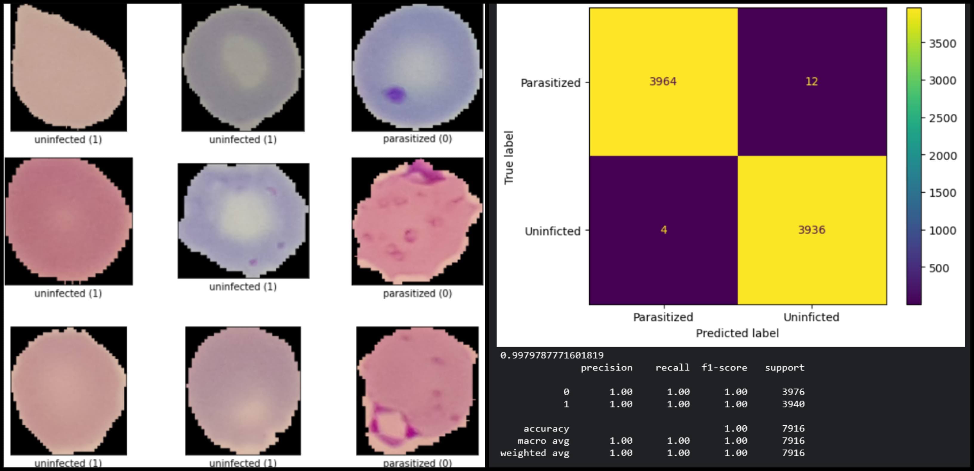
*Fig.1: Data set examples *
Best practices for fine tuning computer vision models
*Fig.1: Data set examples *
For several reasons the model needs to be lightweight and run on an edge device embedded in microscopes. You turn to TensorFlow Hub, an online repository of pre-trained deep learning models, searching for a model that fits the bill. You come across MobileNet V3[3].
MobileNet V3 is a deep neural network architecture designed specifically for edge applications. It is known for its lightweight, high accuracy, and fast inference speed, making it an ideal choice for computer vision at the edge. With your cleaned dataset in hand, you can now fine-tune the MobileNet V3 model to better suit your specific use case.
For our case, I stacked a linear layer with 100 neurons and a classification layer with softmax activation function on top of the pre-trained feature extractor. Moreover, I’ve already set up a simple data pipeline and have my training code in place.
This qualifies me for the next round!
Gaining Insights
My system supports a batch size of up to 248 for this dataset. It is large enough to provide quick iterations so I stick with it.
Starting with my first experiment, I try 2 different optimizers and observe the effects on convergence. Do they influence validation loss a lot? Optimizer is the experimental parameter during this round. However, the* learning rate* is a nuisance parameter, hence I may need to try at least two different values. The number of optimizers and learning rates you choose to test will depend on your computing budget and project goals.
As we mentioned it’s important to observe the learning graphs and not just the success metric.
I start with Adam optimizer, a standard lr=0.003, and train for 10 epochs using early stopping and a simple learning rate reduction scheduler with a factor of 0.3 and patience of 2.
Evaluating on the validation set:
 Best practices for fine tuning computer vision models
Not a bad start…
However, the graphs will reveal more info. Firstly, we observe how the validation loss begins incrementing after epoch 5, indicating overfitting is present. However, since the validation accuracy performs well, I would be tempted to increase the number of epochs and the patience for early stopping, instead. Since the increase in accuracy suggests convergence is still ongoing. Bear in mind that during epoch 8 the scheduler reduced the learning rate.
 Best practices for fine tuning computer vision models
 Best practices for fine tuning computer vision models
Fig 2: Learning graphs. Overfitting or just increase training epochs and reduce early stopping patience?
Best practices for fine tuning computer vision models
Fig 2: Learning graphs. Overfitting or just increase training epochs and reduce early stopping patience?
A quick look at weight histograms, reveals that the early layers of the network don’t change much (fig 3). We can see how they remain mostly stable across epochs. This can reveal a vanishing gradient problem. However, in our case we expect the learning to be concentrated in the last layers.
Indeed, figure 4 shows that MobileNet’s last layers do undergo slight changes, while the classifier (figure 5) is where most of the learning is concentrated on, especially on biases.
 Best practices for fine tuning computer vision models
Fig 3: MobileNet’s first layers remain almost entirely unaffected. We can suppose that there is no need for them to change too much anyway.
Best practices for fine tuning computer vision models
Fig 3: MobileNet’s first layers remain almost entirely unaffected. We can suppose that there is no need for them to change too much anyway.
 Best practices for fine tuning computer vision models
 Best practices for fine tuning computer vision models
Fig 4: MobileNet’s latest layers are fine-tuned and sharper changes in weight values are observed
Best practices for fine tuning computer vision models
Fig 4: MobileNet’s latest layers are fine-tuned and sharper changes in weight values are observed
 Best practices for fine tuning computer vision models
Fig 5: The classifier layer undergoes heavier changes. The learning is mostly focused here.
Best practices for fine tuning computer vision models
Fig 5: The classifier layer undergoes heavier changes. The learning is mostly focused here.
I hope it now becomes clear why inspecting many training graphs is important for deep learning training. They are a very rich source of information.
I then proceed to test whether a bigger learning rate can provide faster convergence without affecting performance. It turns out that lr=0.03 was not a good nuisance parameter value for the Adam optimizer, resulting in suboptimal performance and explosive behavior. It’s interesting how the weights of early layers were severely affected, something we usually do not intend when fine-tuning pre-trained models.
 Best practices for fine tuning computer vision models
Fig 6: Severely affected weights of an early layer in the feature extractor.
Best practices for fine tuning computer vision models
Fig 6: Severely affected weights of an early layer in the feature extractor.
Following a similar procedure for my other experiments I gained enough insights into the problem to design a tight search space for the exploitation phase, where Keras-Tuner will find the most optimal values using Bayesian Optimization.
Automatic Tuning of Pre-trained Models
I will now let the tuning software find the best parameter combination. I define the model and the search space inside the MobileNetHyperModel class and then execute the search with Bayesian Optimization. In my case Keras-Tuner was used, but there are many similar tools available.
I set my computational budget to 10 and let each model train for 10 epochs with early stopping enabled. Now you just have to wait for the algorithm to finish searching. I*f you are constrained by computational budget, you may opt to execute the search on a fraction of the dataset, say 50%, and once you have an optimal model you can train it again on the full dataset. *
 Best practices for fine tuning computer vision models
Fig 7: Example output of Keras Tuner during searching. An optimal model has already been found by trial 3!
Best practices for fine tuning computer vision models
Fig 7: Example output of Keras Tuner during searching. An optimal model has already been found by trial 3!
Finally, I extract the best parameter combination and train the optimal model for 10 epochs. First I evaluate on my validation dataset. Since I am very satisfied with the model’s performance on the validation dataset, and the training graphs look good without any obvious problems, I decide to stop the tuning here and use this model for production.
Before I deploy it, I evaluate it on the test dataset to get an unbiased evaluation. This performance should act as an indication of what to expect while in production.
 Best practices for fine tuning computer vision models
* Fig 8: Evaluation of the final model on the test dataset.*
Best practices for fine tuning computer vision models
* Fig 8: Evaluation of the final model on the test dataset.*
After the model is deployed you will most probably experience performance degradation due to data drifts, so having a baseline is important. Using feedback loops is an effective way to combat the performance degradation of deployed machine learning models.
Final Thoughts
Fine-tuning deep learning models can become pretty tedious and time-consuming. However, results can come faster if you have a pre-defined strategy, a visualization tool, a tuning tool, and of course expertise with deep learning and your underlying field!
In this blog post, we explored a typical case in computer vision. The post was meant to provide some valuable information and act as an inspiration rather than a detailed coding walkthrough.
We worked with a pre-trained deep learning model and fined-tuned it on a custom dataset. We explored some best practices for fine-tuning deep learning models and applied them to fine-tune a lightweight MobileNet computer vision model on an image biology dataset.
REFERENCES
- Deep Learning Tuning Playbook by Google
- Measuring the Effects of Data Parallelism on Neural Network Training. Shallue et al. 2018
- Searching for MobileNet V3. Howard et al. 2019
- Weight Histograms explanation
- Transfer Learning with TensorFlow Hub
- Practical Tutorial on Keras Tuner (Blog post by the author)
Related from Picsellia
Track every experiment
Log metrics, parameters, and artifacts automatically. Compare runs side by side and ship better models faster.
See Experiment TrackingOrganize and version your datasets
Version, slice, and manage datasets with full traceability — from raw images to production-ready splits.
Explore Dataset ManagementStay up to date
Get the latest posts on computer vision, MLOps, and AI delivered to your inbox.
Related articles
From Computer Vision to Industry 4.0: How Scortex Is Shaping Automated Visual Inspection
Discover how Scortex leverages AI and computer vision for automated visual inspection, from defect detection to anomaly detection and real-time insights.

Mastering Data Annotation for AI Projects in 2025
This article will discuss the importance of data annotation in AI and the best practices and strategies for overcoming labeling hurdles.

2025 Trends in Computer Vision: What to Expect
Learn about the upcoming Computer Vision trends in 2025.