How to Train YOLOv5 on a Custom Dataset, Step by Step
We'll show you the step by step of how to easily train a YOLOv5, by using a complete MLOps end-to-end platform for computer vision use-cases.
Picsellia Team
·13 min read
Ready to try this yourself?
Get hands-on with Picsellia. Train, deploy, and monitor CV models from one platform.
Note: The following video was recorded on Picsellia’s previous version, while this current blog article has been updated with Picsellia’s latest interface crand newest MLOps features for computer vision (Updated: 17-March-2022)
As an introduction, we'll briefly walk through YOLO algorithms. For those who don’t know what YOLO is, it’s one of the most known object detection algorithms that has been achieving state-of-the-art results for quite a few years now.
The goal of this tutorial is to teach you how to train a YOLOv5 easily, by using our MLOps end-to-end platform in computer vision. But first, we’ll quickly cover its theory. This article will look as follows:
- Object-detectors evolution
- What is YOLO and how it’s different from other object detectors
- How it performs
- YOLO v5 in depth
- How to train YOLO v5 on your own custom dataset
Let’s get started!
Object-detectors evolution
There are a few types of object detectors, R-CNNs and SSDs.
R-CNNs are Region-Based Convolutional Neural Networks. These are older, and are an example of two-stage detectors. The two stages are, a selective search that proposes a region, this is, bounding boxes that might contain objects; and a CNN used to classify this region. As you can see in the following figure, the two steps are done sequentially, which can take a lot of time.
 How to train yolov5 on a custom dataset
The problem is that R-CNN's first implementation in 2013 was really slow. This left a lot of room for improvement, and that’s what has been achieved in 2015 with Fast R-CNN, and later Faster R-CNN. These replaced the selective stage with Region Proposal Network (RPN), finally making R-CNN an end-to-end Deep Learning object detector.
 How to train yolov5 on a custom dataset
This family of detectors usually throw pretty accurate results, but are quite slow. For this reason, researchers came up with a different architecture called Single Shot Detectors (SSD), which YOLO is part of.
SSD TIMELINE
- 2015: YOLO (You Only Look Once)
- 2016: YOLO 9000
- 2018: YOLO v3
- 2020: YOLO v4
- 2020: YOLO v5
What makes those algorithms fast?
They simultaneously learn the object’s coordinates but also the corresponding classes. They are less accurate than R-CNN but much faster. That’s the philosophy behind YOLO and the many iterations known over the years.
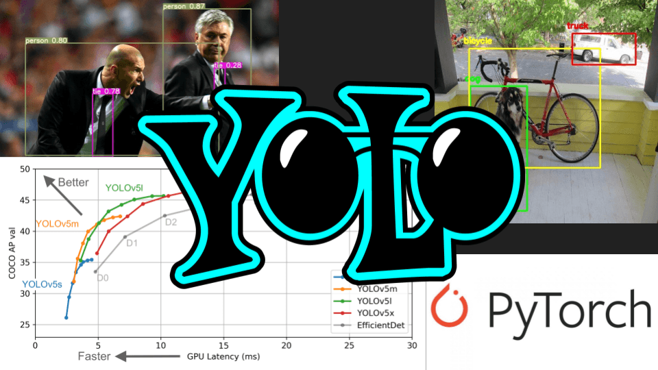
Today we’re going to focus on the last one to date, YOLO v5. As you can see in the following graph, it really performs well, even against efficient debt, which is exponentially slower as you choose a higher version of it.
 YOLOv5 in PyTorch > ONNX > CoreML > iOS
What does performance look like?
Pros
- Much faster than R-CNN-based detectors
- SOTA performance today with YOLO v5
Cons
- Slightly less accurate than R-CNN
As we can see next, there are multiple versions of YOLO v5 itself. It goes from small to extra large sizes, with obvious differences in weight, performance, and latency. This is good news because we can choose a version that is either very fast, but less accurate; or versions that are good compromises between latency and precision, and a heavier version that will perform better.
 How to train yolov5 on a custom dataset
Yolov5 Sizes
How to train yolov5 on a custom dataset
Yolov5 Sizes
Now that we’ve covered a little bit about YOLO and the main differences with other algorithms, let’s train it!
How to train YOLOv5 on a Custom Dataset
For the record, Picsellia is an end-to-end MLOps development platform that allows you to create and version datasets, annotate your AI data, track your experiments and build your own models. What is more, its newest version lest you deploy and monitor your models, and orchestrate pipelines to automate your AI workflows—all in the same place.
If you’d like to learn more about it, feel free to check out our documentation, or schedule a quick call here with our team.
Without further ado, let’s get started!
1. Create the Dataset
This is what the annotation interface looks like. We’ll choose a wine-grape dataset for our object detection project.
 How to train yolov5 on a custom dataset
Picsellia's dataset interface
How to train yolov5 on a custom dataset
Picsellia's dataset interface
We can sort out the dataset this way to see further details, as shown next.
 How to train yolov5 on a custom dataset
As you can see, the dataset is already fully annotated with 5 different classes, corresponding to different types of grapes.
If you click on the “Analytics” tab, you can get a better look of the data distribution and object by image distribution (among other metrics).
 How to train yolov5 on a custom dataset
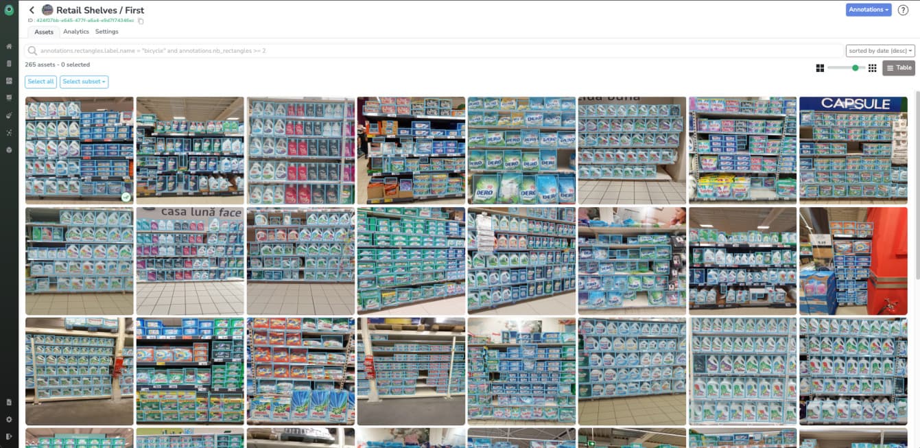
Now, let’s take a look at the annotations. Back to the “Images” tab, we can select all the dataset, or just a subset of the images we want to label.
 How to train yolov5 on a custom dataset
Our platform comes with a pre-annotated system and a robust AI labeling toolbox that let you fully automate your annotations. This way, you can only keep the most accurate ones and optimize your training set.
As we can see next, the dataset is well annotated with every grape inside the bounding boxes.
 How to train yolov5 on a custom dataset
You can select the images or subset you wish, to annotate, accept, reject or interact through comments and mentions with your colleagues. This way, you'll make sure everyone is working on the same data. On a side note, Picsellia also comes with a "Review" system, where assigned collaborators can either accept or reject the labels.
 How to train yolov5 on a custom dataset
Annotation interface
How to train yolov5 on a custom dataset
Annotation interface
Now, for the sake of simplicity, we won’t create a model that can detect all those 5 classes, but rather, an object detector that can detect grapes in general. For that, we'll merge the 5 classes into one that we’ll call “grape”, and create a new dataset version with it.
First, I’m going to select all my images and create a new dataset version with no labels (“Create blank”).
 How to train yolov5 on a custom dataset
Once created, I’ll go back to the “Datasets” tab on the sidebar menu, and see my newest unlabeled version. I can see that I have various versions of my dataset. Now, let’s choose our newest version—“grape-no-label", so we can set up the labels, and merge the different grape classes into just one ("grape")
 How to train yolov5 on a custom dataset 66ed3a44b4b4e5923687095c 62321ace76bdd41247ac733c versions 2520data
Dataset Versions
How to train yolov5 on a custom dataset 66ed3a44b4b4e5923687095c 62321ace76bdd41247ac733c versions 2520data
Dataset Versions
 How to train yolov5 on a custom dataset
Dataset interface - Unlabeled images
How to train yolov5 on a custom dataset
Dataset interface - Unlabeled images
Now, for setting up your labels, go to the tab **“Settings” **on the top screen, and select **“New labels”. **
 How to train yolov5 on a custom dataset
Settings - Configure labels
How to train yolov5 on a custom dataset
Settings - Configure labels
Next, choose your annotation class–in this case, Object Detection–, name it and add it as follows. Then, just hit “Create labels”.
 How to train yolov5 on a custom dataset
Now it’s time to merge our labels!
We’re gonna import the annotation from our old dataset into this version, and merge the 5 different labels into just one.
For that, click on “Annotations”, where we’ll select the version of the dataset we’d like to import our labels from. In this case, it’s the dataset called “first” that contains the 5 different grapes.
 How to train yolov5 on a custom dataset
Choose the output label “grape” as shown below, and select each one of the annotations to import as “grape” by clicking their checkboxes. Next, click “Execute instructions”.
 How to train yolov5 on a custom dataset
If we go to the **“Settings” **tag, we can see that our label is well defined as just one “grape”, and see it has the 3,920 objects.
 How to train yolov5 on a custom dataset
Back to the Dataset interface (“Images” tab), we can see just one label.
 How to train yolov5 on a custom dataset
If we take a look at the annotations, we can observe that all our bounding boxes contain all different types of grapes, now labeled just as “grape”.
 How to train yolov5 on a custom dataset
Now, let’s get down to the real business: to train a YOLOv5 on this dataset.
2. Set Up The Training
We’re going to create a new project named “yolo-grape-test”, that uses this dataset and organizes my trainings.
 How to train yolov5 on a custom dataset
At Picsellia you also have the option to invite team members to your project to work on the same data (we’re going to skip it for this tutorial).
 How to train yolov5 on a custom dataset
Invite your teammates to collaborate
How to train yolov5 on a custom dataset
Invite your teammates to collaborate
Just for the record, on the “All Projects” tab, on the sidebar menu, you’ll see all your projects stored in one single place.
 How to train yolov5 on a custom dataset
Project Hub
How to train yolov5 on a custom dataset
Project Hub
Now, let’s check our project. At this point, the project is pretty empty, so we’re going to attach the dataset we just created to this project, for which we’ll click “Open Datalake”.
 How to train yolov5 on a custom dataset
We then select our desired project, “Embrapa-wine-grape”.
 How to train yolov5 on a custom dataset
And we want to choose the “grape-one” version.
 How to train yolov5 on a custom dataset
Our dataset is now well attached!
 How to train yolov5 on a custom dataset
Next, before creating our experiment, let’s take a look at the Models section of Picsellia.
 How to train yolov5 on a custom dataset
Picsellia's models
How to train yolov5 on a custom dataset
Picsellia's models
On this page you can find every model that we uploaded that are base architecture that you can use to kickstart your experiment, as shown below.
 How to train yolov5 on a custom dataset
Model Registry
How to train yolov5 on a custom dataset
Model Registry
For our experiment, we’re going to use the YOLOv5-m model, for the sake of the speed of training. You can use this model out of the box, meaning, you don’t have to do anything, just select them.
Now it’s time to go back to our project, and create our experiment using this pre-trained YOLOv5-m model.
Once there, we’re going to run our experiment with UI.
 How to train yolov5 on a custom dataset
This is going to be the first version of our training, named “v1”.
 How to train yolov5 on a custom dataset
And, on the second step, we’re going to choose the base architecture model from my “Organization HUB”. In this case, YOLOv5-m.
 How to train yolov5 on a custom dataset
To run YOLOv5-m, we just have to set up two parameters. The number of steps (or “epochs”) and the batch size.
For this tutorial, and to show it quickly, we’re just setting up 100 epochs. As we will run it in Colab, we’re going to set up a small batch size, 1, just for the test; and run it on a large hardware later.
 How to train yolov5 on a custom dataset
Lastly, we select our dataset.
 How to train yolov5 on a custom dataset
Then we create the experiment, and we’ll see the experiment overview. We have our base model, our attached dataset, and our parameters are all set up.
 How to train yolov5 on a custom dataset
The beauty of Picsellia is that in the **“Launch” **tab, we can choose different ways to launch our experiments.
 How to train yolov5 on a custom dataset
We’ll be launching it with Google Colab, so by clicking there, we’ll access a preconfigured Jupyter notebook with all things needed to train a YOLOv5. I’m going to quickly show you all steps required to launch the training.
3. Launching the Training
First, we have to install the Picsellia package, along with the Picsellia YOLOv5 package. In this library, we’ve packaged the whole Pytorch implementation of YOLOv5.
 How to train yolov5 on a custom dataset
We have to import the packages along with Pytorch, os, subprocess, etc.
 How to train yolov5 on a custom dataset
We have to leverage the experiment system of Picsellia to get all the files we have from our pre-trained work and the parameters, so with the checkout we can get everything on the instance.
 How to train yolov5 on a custom dataset
 How to train yolov5 on a custom dataset
Then we need to download the annotations and images.
 How to train yolov5 on a custom dataset
We set up a directory that will store our images and annotations.
 How to train yolov5 on a custom dataset
 How to train yolov5 on a custom dataset
We then have to generate a .yaml that will contain the label map along with the directory, the path of the training and test images.
 How to train yolov5 on a custom dataset
Next, we have to set up the hyperparameters that will be used for training, so the only things we have to give are the parameters we set up from Picsellia, the label map, and the experiment name.
 How to train yolov5 on a custom dataset
And next, we can finally launch the training!
 How to train yolov5 on a custom dataset
 How to train yolov5 on a custom dataset
We already launched it in order to show it to you, because it can be pretty slow on a Jupyter CPU notebook. But, as you can see, the training is going pretty well.
 How to train yolov5 on a custom dataset
And, everything is sent back to Picsellia, live!
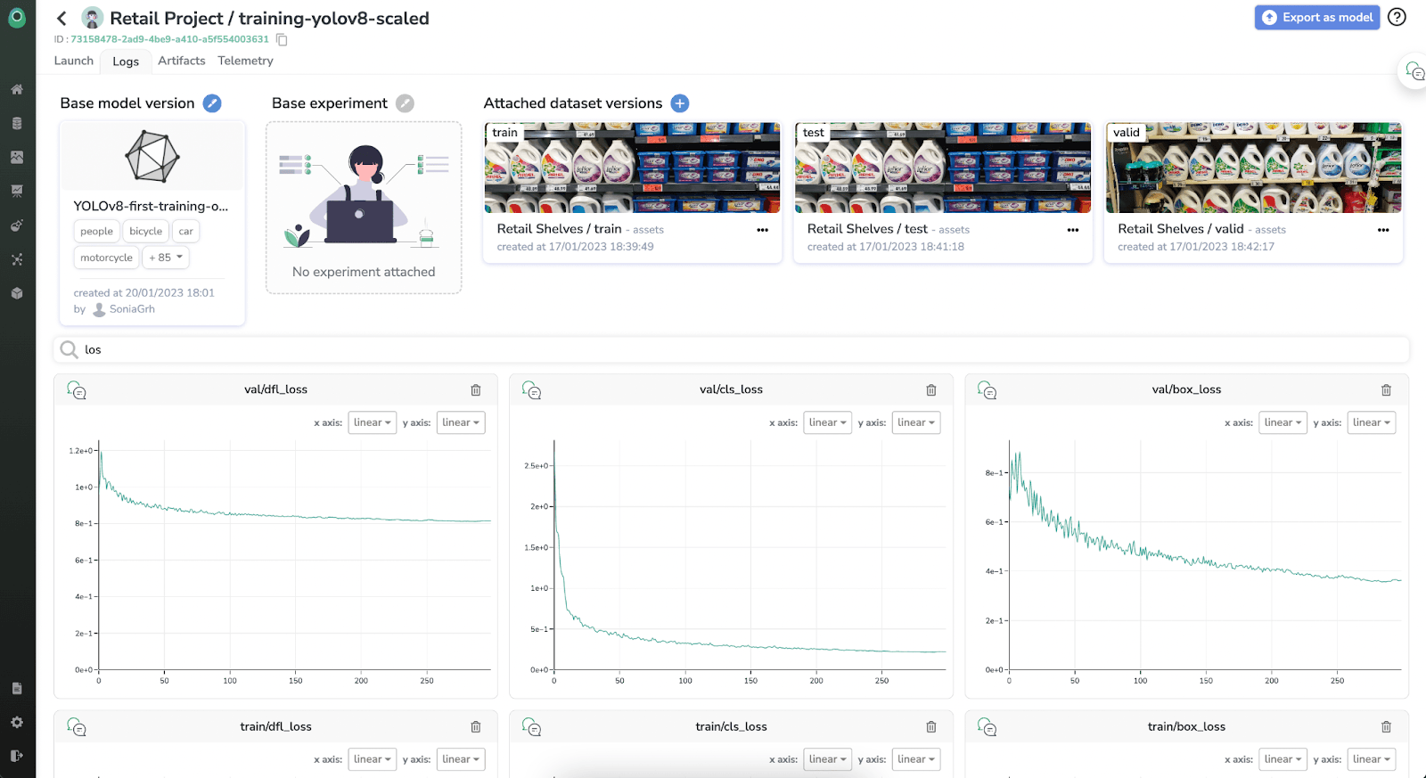
As you can see next, I already have my training metrics live on the platform. If I refresh the page, I should have some more values, with the new epochs.
4. Check the Results
Now, as it’d be too long to wait for the training to finish, and to show you real results with a longer training, I set up another training that I will show you next.
 How to train yolov5 on a custom dataset
This one training has 1000 epochs as was trained on NVIDIA v100 GPUs. As you can see, the metrics are pretty good.
 How to train yolov5 on a custom dataset
We do have problems with our loss here–we should investigate it later–, but as you can see, it does converge a little bit.
 How to train yolov5 on a custom dataset
Now, let’s see results with evaluation on real images from our dataset. For this, I logged the images from my evaluation on different batches of images.
 How to train yolov5 on a custom dataset
I downloaded one of these images. We do already have some great results for our great detection algorithm!
 How to train yolov5 on a custom dataset
As an example, if we did just 1000 epochs (or “steps”) of training, the whole training process could take up to 4 hours. While, for our original test, where we only set up 100 epochs, that could take only a few minutes.
 How to train yolov5 on a custom dataset
If we go check the files of our experiment, we have successfully uploaded all the files needed to resume our training later. We need the config file, which is the yaml; a checkpoint file for hyperparameter; and another checkpoint file which is the pytorch weights.
 How to train yolov5 on a custom dataset
Now, we can resume our training whenever we want and iterate over and over on our experiments easily using Picsellia!
If you’d like to try Picsellia and leverage our latest MLOps features (model deployment, monitoring, automated pipeline orchestration, and more), request your trial here!
Related from Picsellia
Train models your way
Use pre-built pipelines for YOLO, SAM2, and more — or bring your own code with PyTorch, TensorFlow, or Hugging Face.
Explore the AI LaboratoryTrack every experiment
Log metrics, parameters, and artifacts automatically. Compare runs side by side and ship better models faster.
See Experiment TrackingStay up to date
Get the latest posts on computer vision, MLOps, and AI delivered to your inbox.
Related articles
Train and integrate YOLOv8 with Picsellia in just a few minutes
In this tutorial, we will provide you with a detailed guide on how to train the YOLOv8 object detection model using Picsellia.
How to train YOLOv8 on a custom Dataset
YOLOv8 is the most recent edition in the highly renowned collection of models that implement the YOLO (You Only Look Once) architecture.